A few months ago I got tired of commuting to the local hacker space so I bought a cheap 3D printer to use at home. Like any good neophyte, I printed quite a few precooked models before getting the itch to design some of my own.
The biggest hurdle was that I couldn’t find good modeling software to run on Linux. I tried FreeCAD and Blender but found them hard to approach. I eventually stumbled upon OpenSCAD which I ended up absolutely loving. So hopefully this is the first of at least a few posts where I dive into some of the techniques I’ve learned.
There’s obviously a lot of useful things you can make with a 3D printer. For my first project, I decided on a spice rack for two reasons:
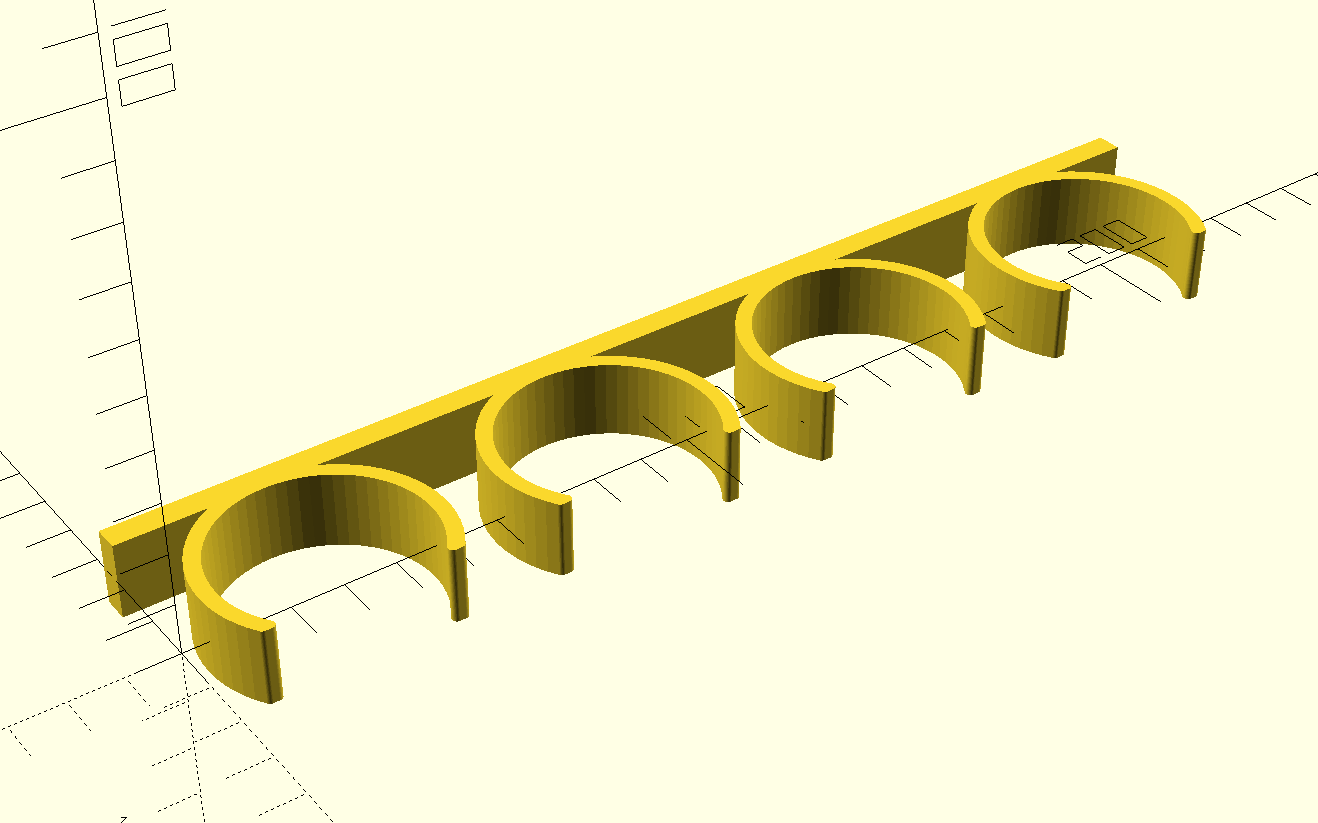
Here’s the final design for reference:
I’m not really an expert at 3D modeling so I won’t say much about the theory. But based on my limited research, I found OpenSCAD’s marriage between declarative scripting and constructive solid geometry (CSG) to be a wonderfully elegant combination.
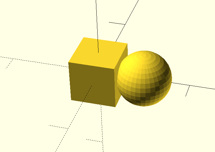
The premise behind CSG is that there are a limited set of 2D and 3D primitives such as squares, circles, spheres, cylinders, cubes, etc. which can be combined with with boolean operators to yield complex geometries. For example, with the following code, you can take the union of a cube and a sphere to yield a cube-sphere fusion:
union() {
    cube([5, 5, 5], center=true);
    translate([5, 0, 0])
        sphere(r=3);
}
Expressions are not limited to the top level – they can be arbitrarily nested. Consider this following example:
module ring() {
    difference() {
        circle(r=10);
        circle(r=5);
    }
}

linear_extrude(15) {
    union() {
        translate([15, 0, 0]) ring();
        ring();
    }
}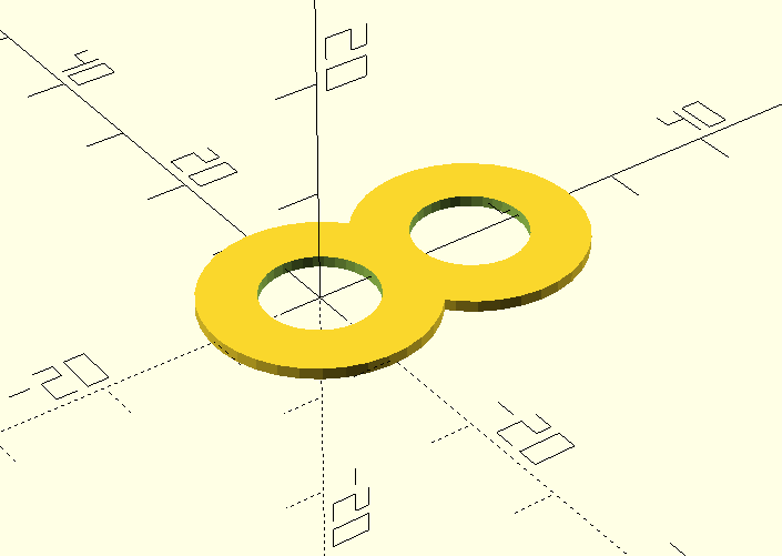
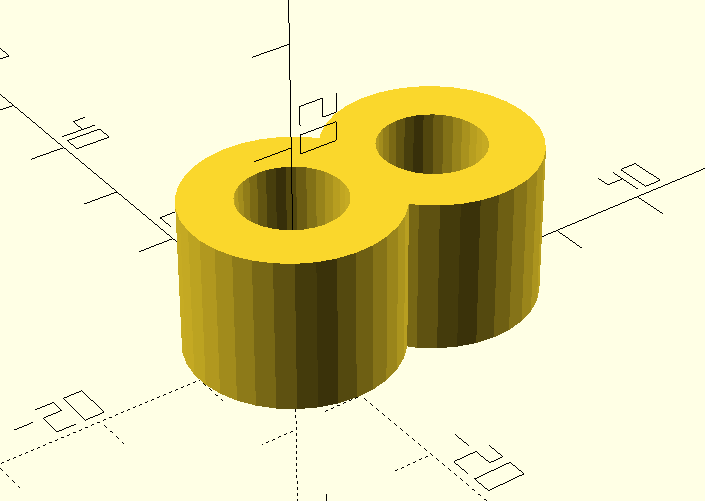
The basic idea is we first create two rings, one next to the other. We then take the two rings and join them with a union. Finally, take the union and extrude along Z axis to create the binocular shape on the right above.
The other new technique here is a module. A module,
taken in the context of C/C++ like languages, is essentially a macro. We
don’t use any parameters in the module here, but we could have.
Knowing these basics, we move onto the rack design.
To start, we create the backboard:
translate([(225/2), 25, 0])
    cube([225, 5, 15], center=true);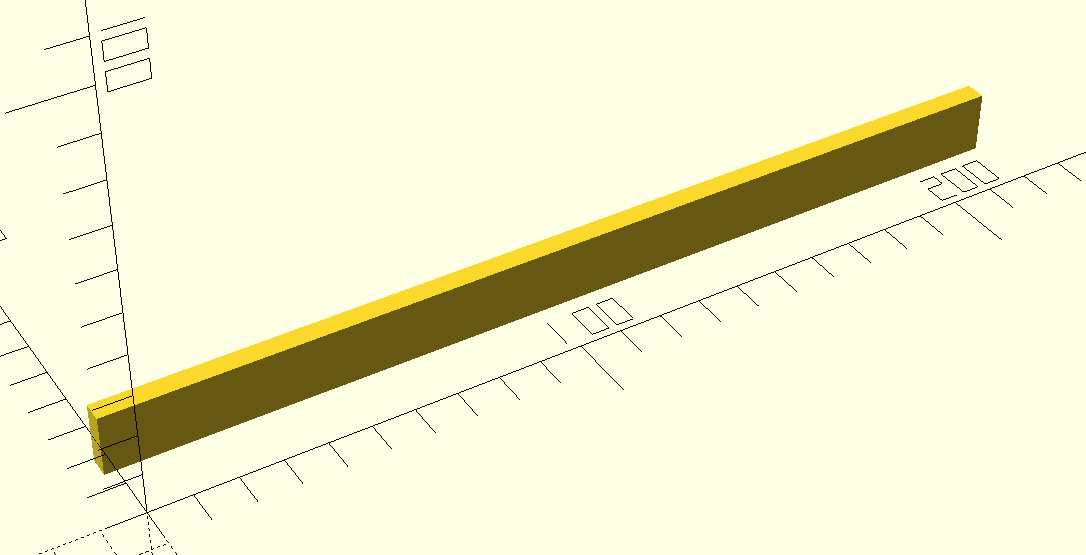
We translate the backboard a bit so that it’s length is easier to eyeball on the X axis and so it’s arms are more easily positioned on the Y axis. Note that OpenSCAD is unitless but my slicer (Cura) interprets the units by default as millimeters.
Next we create the arms:
inner_radius = 20;
outer_radius = inner_radius + 3;

module arm() {
    difference() {
        intersection() {
            circle(outer_radius);
            translate([0, 7.8, 0])
                square([500, 41], center=true);
        }
        circle(inner_radius);
    }
}

for (i=[0:3]) {
    translate([i*56.5 + 28, 2, 0])
        #arm();
}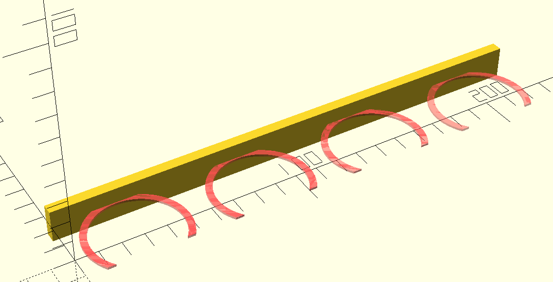
The arms follow a similar design to the examples above. We make each
arm by intersecting two circles and slicing off the end so the spices
can fit. And instead of making one, we make four by using a
for loop.
One practical tidbit here is we lexically prefix each arm with
# to give it a different render color. This is useful for
quickly eyeballing changes to your model. In this case, we’ll be using
it to illustrate the changes from the previous code snippet.
Once we have the 2D arms, all that’s left is to extrude them to the appropriate height:
module arm() {
    #linear_extrude(15, center=true) {
        // Previous contents of `arm()`
    }
}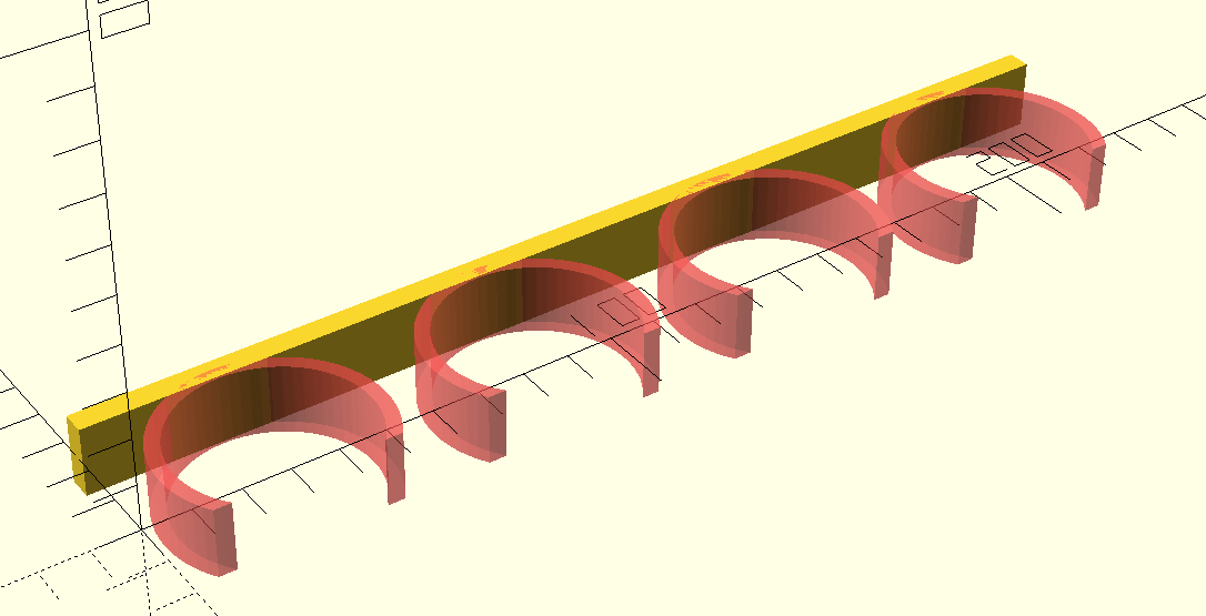
At this point we have a functional model. In fact, this is what I have printed and installed in my cabinets. However, there’s still one small improvement we can make: the tips of the arms. The tips are slightly sharp and could use some rounding out. To achieve this, we’ll use a Minkowski Sum.
Minkowski sums are hard to explain through text but surprisingly easy to understand with a visualization. In the previously link, the animation demonstrates that the sum of two nodes involves running the child node around the edges of the parent node and adding the shape that the child node’s motion creates to the parent node.
In our case, we’ll run a small circle around the edges of the arm while also subtracting an additional unit off the inside and outside to keep the final dimensions roughly the same. The end result is the sharp edges are rounded out but the smooth parts remain unchanged.
In code, this looks like:
minkowski_radius = 1;

module arm() {
    linear_extrude(15, center=true) {
        minkowski() {
            difference() {
                intersection() {
                    circle(outer_radius-minkowski_radius);
                    translate([0, 7.8, 0])
                        square([500, 41-minkowski_radius], center=true);
                }
                circle(inner_radius+minkowski_radius);
            }
            circle(minkowski_radius);
        }
    }
}
With this we arrive at the model displayed in the beginning of this post.
For completeness, the following is the physical result. As I mentioned earlier, the physical model doesn’t yet have the rounded edges (the 3M adhesive strips are surprisingly expensive!). So you’ll have to use your imagination a little here.
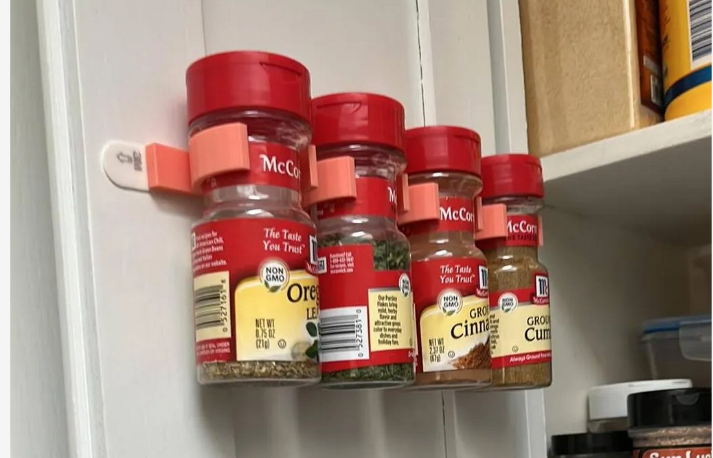
Obviously this is not a complicated geometry. In fact, a (real) engineer friend of mine was timed creating a similar model using professional tooling and it took him about 90 seconds. Despite that, I still think this was a really enjoyable process. I particularly love how the entire language fits on a small cheat sheet – something unimaginable for industrial grade tools. So I suppose my preference for elegance over practicality is why he’s a real engineer and I’m not.